Single vertical fault example
The following example shows how to extract and mesh a fault from a 3D model.
The purpose of this example is to be interactive to better understand the step-by-step workflow.
However, up to the medial axis computing (see this section), all the steps can be performed in a single call to the script get_medial_axis.py.
This file is the single strike-slip fault example provided in the article “3D reconstruction of complex fault systems from volumetric geodynamic shear zones using medial axis transform” and can be found in this repository.
You can familiarize yourself with the mesh by loading it in Paraview.

Step 1: Extrude mesh vertically
This step is optional, but working with extruded meshes can be easier to extract faults. In this example we will extrude the surface of the mesh in the \(y\) direction, but note that this process can be done in any of the three directions.
To do so we will use a YAML file with the following content:
model:
  file: "Models/single_fault-cellfields-e2.vts"
  output: "Faults_output"
  fields: ["e2","xi"]
  e2_key: "e2"

extrusion:
  - name: "ymax"
    nsteps: 5
    dx: 1.0e4
The block model specifies the input mesh file, the output directory,
and optionally the fields to be extruded and the key of the strain-rate second invariant field.
The extrusion block specifies the extrusion parameters.
In this case, we are extruding the mesh in the \(y\) direction starting from the top boundary,
with 5 steps and a step size of 10 km.
Additional extrusion can be done in the \(x\) and \(z\) directions
by adding them to list such that:
extrusion:
  - name: "ymax"
    nsteps: 5
    dx: 1.0e4
  - name: "ymin"
    nsteps: 3
    dx: 5.0e4
  - name: "xmax"
    nsteps: 1
    dx: 1.0e4
  - name: "xmin"
    nsteps: 2
    dx: 2.0e4
  - name: "zmax"
    nsteps: 1
    dx: 1.0e4
  - name: "zmin"
    nsteps: 1
    dx: 1.0e4
Then, the extrusion can be performed by running:
$ python scripts/mesh_extrude.py -f path/to/yaml/file/extrusion.yaml
After this step, you should obtain a new mesh file single_fault-cellfields-extruded.vts in the output folder.
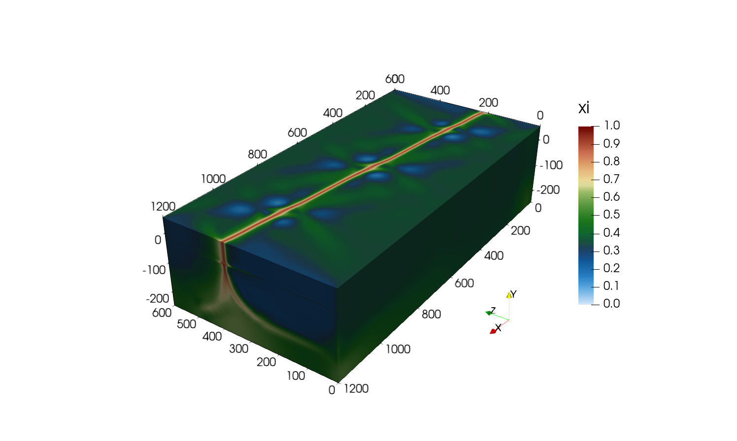
Step 2: Extract shear zone envelope
This step consists of obtaining the envelope of the shear zone.
Using Paraview, load the extruded mesh (or the original mesh if no extrusion was performed) using
file -> open -> Faults_output/single_fault-cellfields-extruded.vts.
Step 2.1: Compute the field xi
If you provided the e2_key in the YAML file used for the extrusion, you should have a new field named xi
on the mesh.
If you need to calculate it again or if you are working with the original mesh, you can use the Calculator or the Python Calculator filter
to apply the following expression:
The following block shows the expression you can use in the Python Calculator filter:
import numpy as np
xi = (
  ( np.log10(e2) - np.min(np.log10(e2)) ) /
  ( np.max(np.log10(e2)) - np.min(np.log10(e2)) )
)
return xi
Step 2.2: Convert cell data to point data
The strain-rate and thus the new field xi are, in our case, defined as cell data.
To extract the envelope of the shear zone, we will first need to convert the cell data to point data using
Filters -> Cell Data to Point Data.
You should obtain the following:
Step 2.3: Extract the envelope
Once the field is converted to point data, apply Filters -> Contour to the mesh and set the contour value to
0.8 on the xi field.
You can play with that contouring value to see how it affects the envelope.
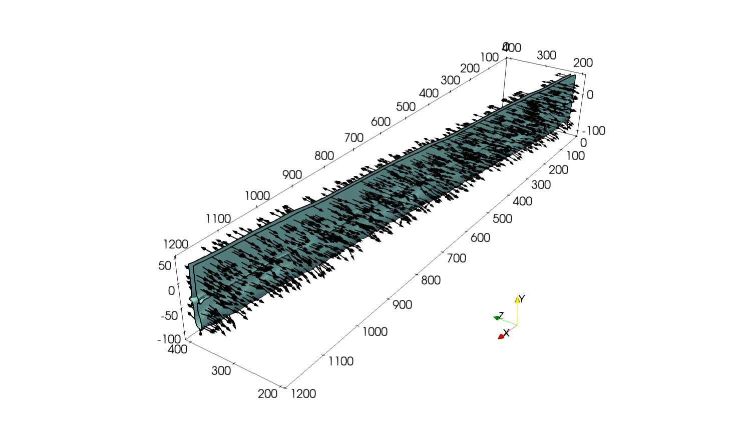
Step 2.4: Compute the normals
Next, it is required to get the outward pointing normals of each point of the envelope. Depending on the Paraview version you execute, the normal vectors may have already been generated when applying the contour filter.
In any case you can generate them by applying the Filters -> Surface Normals or Filters -> Generate Surface Normals
depending the Paraview version.
Ensure that the normals are pointing outwards by visualizing them with the Glyph filter.
If it is not the case, the normals can be inverted using the Flip normals option in the filter generating the normals.
Once done you should have the following:
Finally, save the envelope mesh using File -> Save Data and use a VTK like format.
Note
During the saving process you can select the fields to save, in our case we only need the Normals field.
This functionality is particularly useful to save space disk when working with heavy data.
For the next step, we will assume that the file is saved as Faults_output/single_fault-cellfields-contour.vtk.
Step 3: Compute the medial axis
To compute the medial axis of the fault, we first define a YAML file with the following content:
contour_file: "Faults_output/single_fault-cellfields-contour.vtk"
medial_axis:
  radius_ma: 1.0e4
  get_eigv_cov: true
  radius_cov: 25000.0
The option contour_file specifies the input mesh file.
The block medial_axis specifies the parameters for the medial axis computation.
The radius_ma is the initial distance in distance units of the data contained in the file, here in metres, at which the medial axis computing algorithm starts.
This value should always be greater than the width of the shear zone.
The radius_cov is the radius of the sphere in which points are considered to compute
the covariance matrix at each individual point.
In this example we will not use the covariance matrix analysis given the simplicity of the fault geometry.
Then, the medial axis can be computed by running:
$ python scripts/get_medial_axis.py -f path/to/yaml/file/medial_axis.yaml
After this step, you should obtain a new mesh file in the data folder.
If you used the same naming convention as in the example, the file should be named Faults_output/single_fault-cellfields-ma.vtp.
Note
All the steps presented from section 1 to 3 can be performed in a single call to the script get_medial_axis.py.
To do so, you can use the following YAML file:
model:
  file: "Models/single_fault-cellfields-e2.vts"
  output: "Faults_output"
  fields: ["e2","xi"]
  e2_key: "e2"

extrusion:
  - name: "ymax"
    nsteps: 5
    dx: 1.0e4

contour:
  flip_normals: false
  isovalue: 0.8
  field_name: "xi"

medial_axis:
  radius_ma: 1.0e4
  pca_method: "sphere"
  radius_cov: 25000.0
Then, the medial axis can be computed by running:
$ python scripts/get_medial_axis.py -f path/to/yaml/file/medial_axis.yaml
This will automatically save the extruded mesh, the contour and the medial axis in the output folder.
Step 4: Mesh the fault
Step 4.1: Load the medial axis mesh
Start by loading the medial axis mesh in Paraview using file -> open -> Faults_output/single_fault-cellfields-ma.vtp.
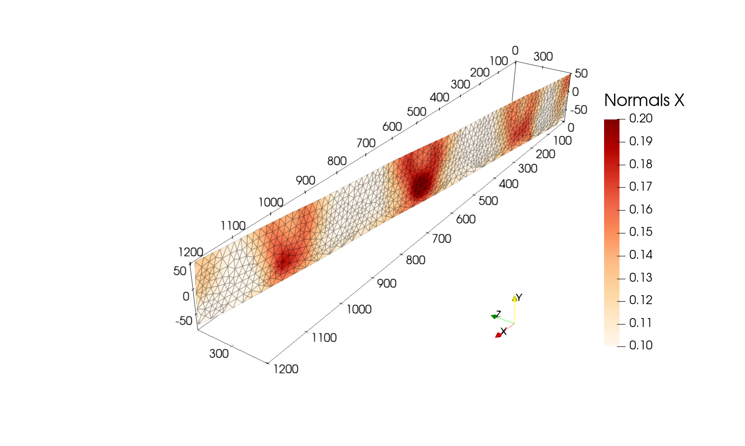
If you display the field eigv_0 and its X component you should obtain the following:
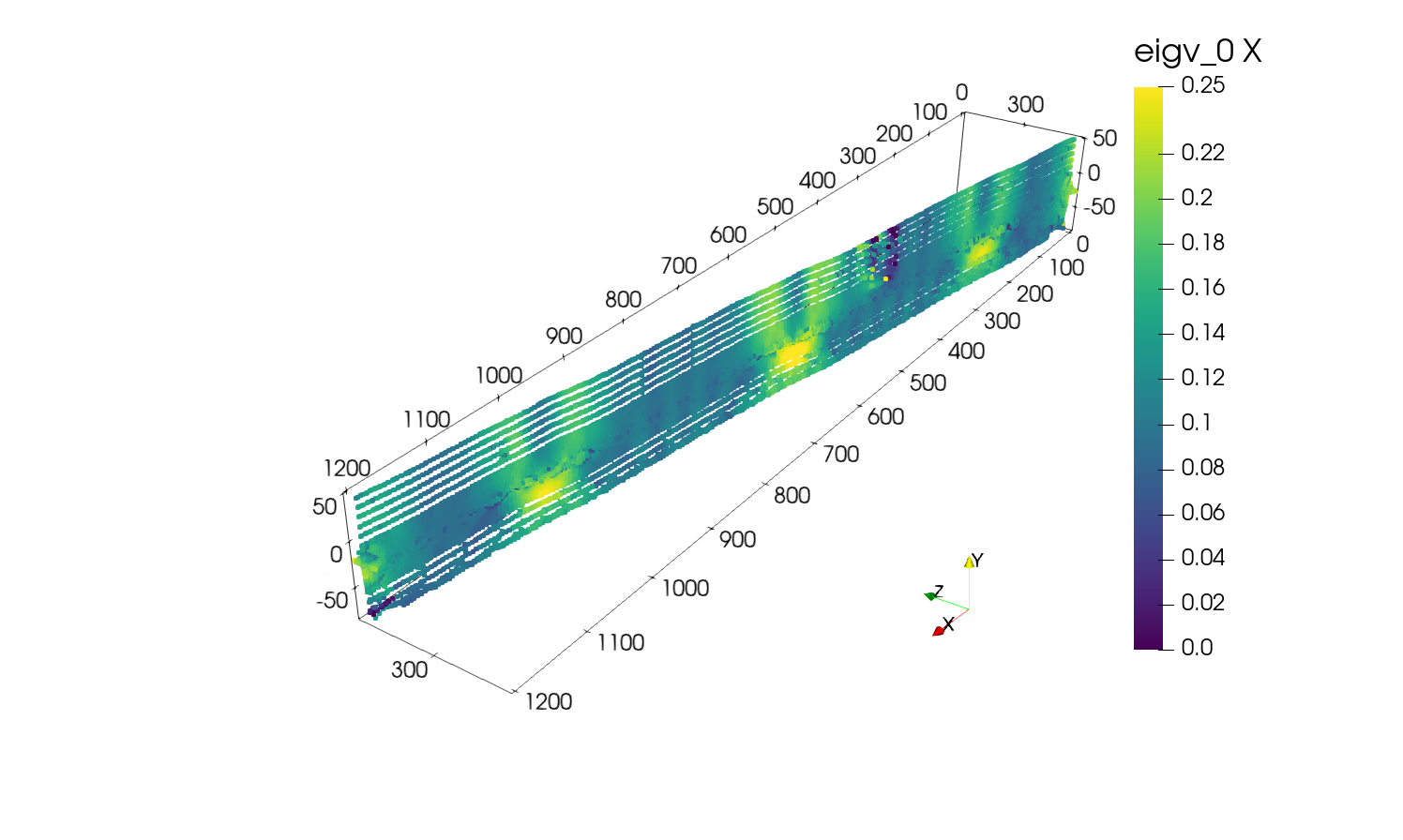
Step 4.2: Delaunay triangulation
Next, apply the Filters -> Delaunay 2D to the medial axis points set.
You can play with the Projection Plane Mode and the Tolerance to see how it affects the mesh.
In this example we will use Best-Fitting Plane and a tolerance of 1.0e-2.
This should result in the following mesh:
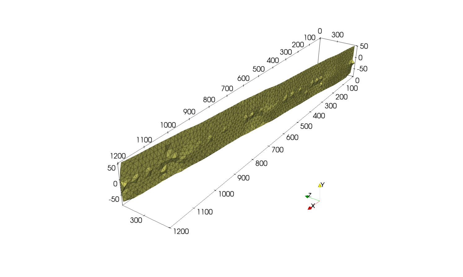
Step 4.3: Smooth the mesh
Once done, we will apply Filters -> Smooth to the mesh to obtain a smoother fault representation.
Again, you can play with the number of iterations to see how it affects the mesh.
In this example we will use 500 iterations, if you compute the normal vectors of the mesh using Filters -> Surface Normals the resulting fault surface should look like:
Finally, save the fault mesh using File -> Save Data to the desired format.
To go further
Note that with further processing, we can interpolate values from the original mesh to the fault mesh to get the stress on fault, the slip rate, etc…
In this example, we processed a model with a single vertical fault, but the same process can be applied to more complex fault geometries as shown in other examples.